Global Optimizer
Overview
Global optimization searches the entire solution space of a given problem to get the best possible match to a set of desired conditions. Our solver takes your target kinematic curves and a set of boundary conditions on the points and searches for the best possible configuration.
As with most mathematical optimizations the boundary conditions have a very strong influence on the outcome and should be set carefully and specifically to your desired outcome. Some good strategies are:
- Allow enough freedom in the boundary conditions. For example allowing only a single point to move or restricting point limits to only a very small distance will result in the total solution space being quite small and likely similar to the starting conditions. This may prevent any close solution from being found.
- Restrict boundary conditions where needed . Restrict your boundary conditions to realistic limits to prevent the solver honing in on unrealistic point positions (such as pivots behind the axle). Sometimes it can be helpful to run several low resolution studies and progressively restrict point movement in line with your intended design direction.
- Run more low resolution solves . Solve times are much quicker for lower resolutions solves but not necessarily less accurate. It is almost always advantageous to run several fast solves to understand where the results are being driven and altering boundary conditions as needed before further optimization.
Activate Solver
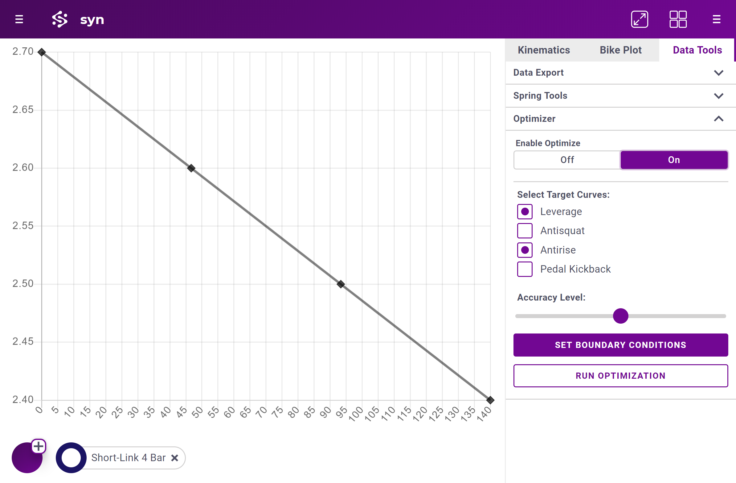
The solver must be activated from the Data Tools tab of the Right Sidebar. Once enabled the target curve selectors will be displayed.
A study is run with respect to the currently selected bike. Once a bike is loaded and at least one target curve is activated the Run Optimization and Set Boundary Conditions buttons will be visible.

Set Target Curves
Enable Targets
Targets curves can be set for the 4 primary kinematic metrics of Vertical Leverage, Antisquat, Antirise, and Pedal Kickback. Select the target or set of targets you want to use from the list under the Optimize heading of the Data Tools tab. A default target curve will be generated for each selection and be visible on the plot as a grey spline with black point handles.
Modify Targets
Each target curve is set by dragging the black diamond Control Handles on the spline. To add an additional handle double click on the target curve. To delete a handle double click on it. The required shock travel for a given leverage curve will be automatically calculated by the solver. Because each target curve is set independently it is important that all curves have very close to the same max wheel travel.
Targets are global to the application and not associated with a particular loaded bike.
Target Weighting
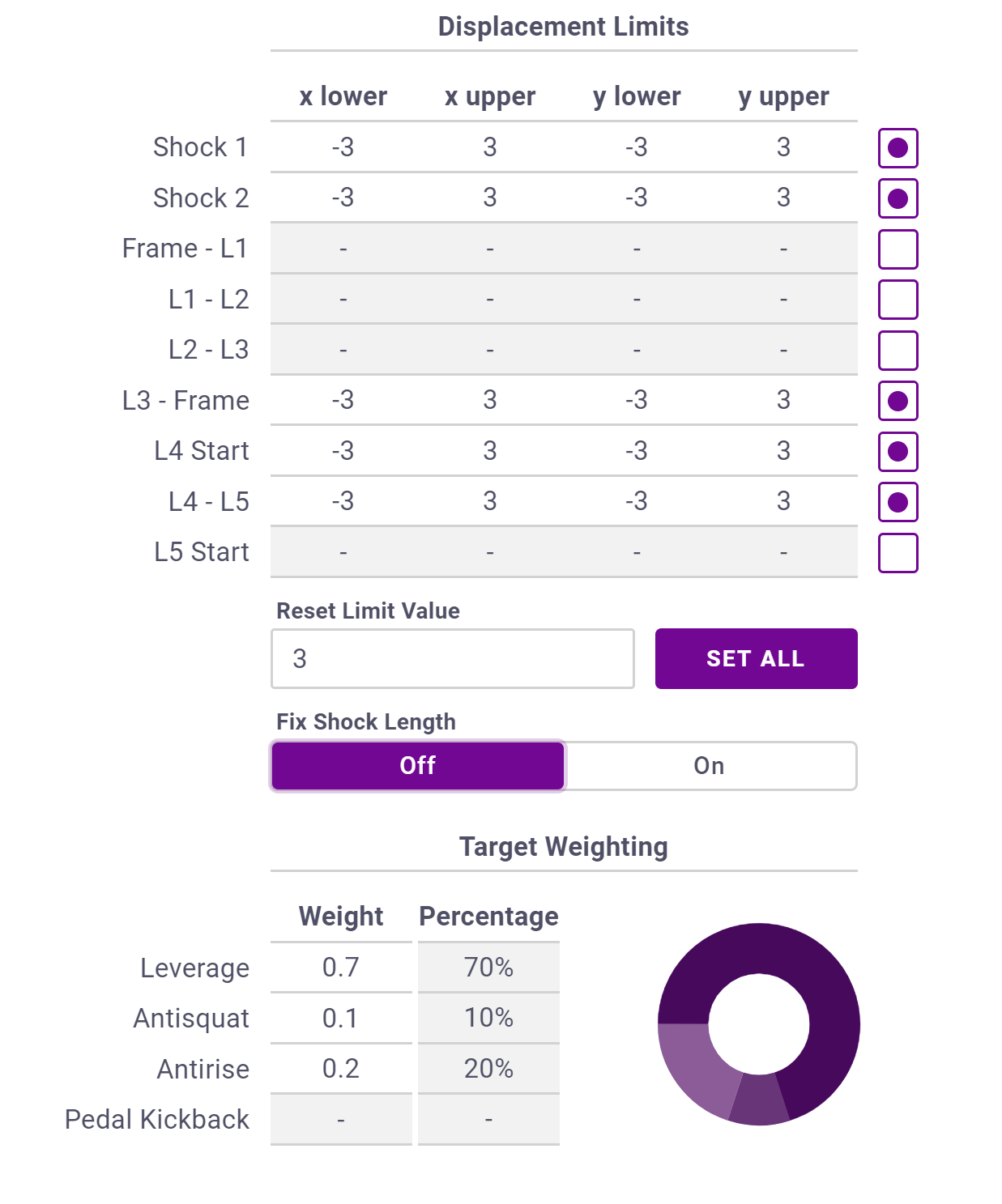
Target weights are set from the Boundary Conditions panel opened by pressing the Set Boundary Conditions button. See the figure for Boundary Conditions below for reference.
A higher weight for a curve will force the solver to give more value to solutions that are closer to that curve at the expense of the other target curves accuracy. This essentially tells the solver how to compromise between two solutions where one result is closer to the target curve but another is further away. The target weights are always sent as percentages but can be entered in any form. The given percent weight is calculated as the input value divided by the sum of all the input values. Percent weights are shown on the pie chart for visual reference.
In general leverage should be given a higher target weight that other targets as leverage curve shape has a much larger impact on bike performance.
Set Boundary Conditions
Once a minimum of one bike is loaded and a target curve is selected the Boundary Conditions panel can be opened by pressing the Set Boundary Conditions button.
Adjust Boundaries
To allow the solver to move a point during the study click the Selector for the associated row. The upper and lower bounds for the points x and y position can then be set. The boundary values set are the maximum possible displacements from the initial point position.
To reset all boundaries to a given number the Reset Limit Value input can be set. Clicking Set All will set a symmetric limit equal to the Reset Limit Value on every point.
Shock Position
The shock position can be set using two methods. The first method is setting a point boundary condition for each end of the shock. This will allow each point to move independently with the total shock length (shock length + shock extension length) changing as needed. This is useful for bikes that use shock extensions and have flexibility in the total shock length.
For bikes where the shock length is a fixed parameter the shock position can be adjusted using a point on one end and an angular range the shock can rotate though. By selecting Fix Shock Length the solver is set to use the specified angular limits and the positional boundary conditions on shock point 2.
Submit Study
Once the target curves and boundary conditions are set the study can be submitted. The currently selected bike is used as the initial conditions for the solutions. Only points are moved; no linkage layout changes are made by the solver.
The accuracy of the study can be set using the Accuracy Level slider. In general no more that 50% is required and higher values will only add time to the solution without increasing accuracy.
Once the solution has been submitted no action is required. When solver is done the result will be sent back through the in-app messaging service viewable through either the navigation menu or the Error Ball. Clicking Accept Bike will load the result into the workspace with a message symbol prefixed to the model name.
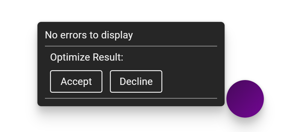
The solver is fully separate from the main application and results will still be processed and sent to the users message inbox if the application is closed.